Probability calibration: why 60% must really mean 6 matches out of 10

Accuracy != calibration

Accuracy measures the number of correct predictions. Calibration measures the statistical honesty of probabilities. A model can be accurate but poorly calibrated, or the opposite.

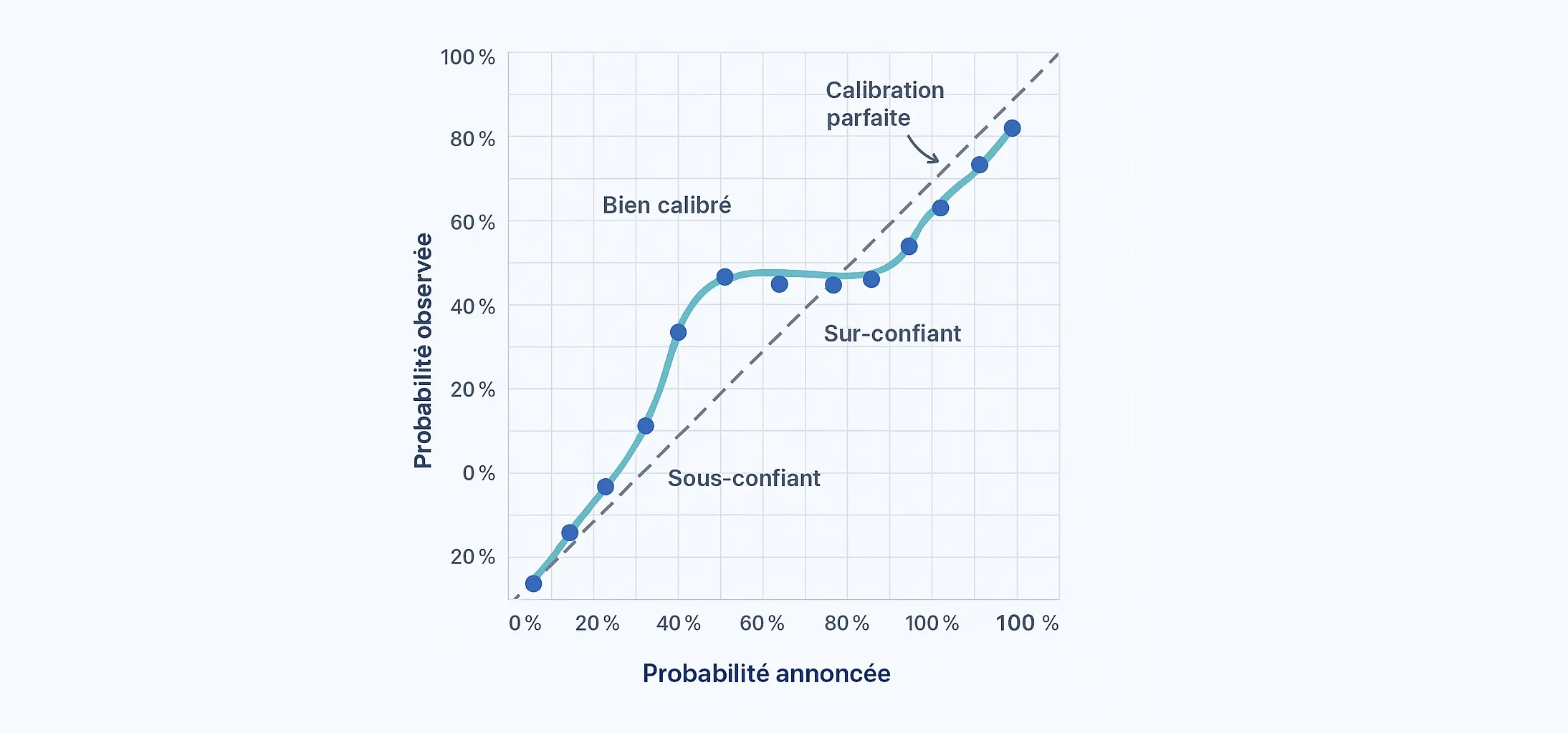
• Well calibrated: 70% announced -> ~70% observed
• Overconfident: 70% -> ~63% observed
• Underconfident: 70% -> ~76% observed

A simple thought experiment helps. Two models may post similar raw hit rates on a 1X2 dataset, but if one keeps publishing inflated 70% probabilities that behave like 60% outcomes, it is much harder to trust in practice. Calibration exists to measure that honesty gap.

Reliability metrics

Brier Score

The Brier Score measures the squared error between probability and actual outcome. It heavily penalizes unjustified certainty.

LogLoss

LogLoss is particularly sensitive to highly confident mistakes. It is useful for detecting overconfidence.

Reliability curve

Probabilities are grouped into bins and compared to observed frequencies. The diagonal represents perfect calibration.

In practical terms: Brier looks at average probability error, LogLoss punishes unjustified certainty, and the reliability curve checks whether a published number behaves like its stated level inside the relevant 1X2 dataset.

Why calibration must be tracked over time

Leagues evolve, styles change, refereeing evolves as well. Without regular recalibration, a model can remain "good" while gradually becoming misleading.

This logic is detailed in the algorithm journal .

This is also why raising a threshold is not the same thing as recalibrating. A threshold changes selection. Recalibration changes the honesty of the displayed percentage itself.

Readers often confuse a cleaner shortlist with a better probability engine. Filtering may improve comfort, but only calibration tells you whether the displayed number still behaves like its label over time.

How to read a probability properly

• a probability is an expected frequency, not a promise
• calibration asks whether the published percentage is honest, not whether the favorite wins often
• recalibration can improve LogLoss and ECE without improving raw accuracy

This is why calibration belongs to probability reading, not only to model engineering. If the percentage itself is misleading, every downstream interpretation becomes weaker, even when the match commentary sounds persuasive.

Concrete calibration example: metrics, bins and draw structure

On the 133,160-row 1X2 production pipeline, the adjuster moves LogLoss from 0.657 to 0.647 and ECE from 0.094 to 0.082. That is the core calibration proof: published probabilities become more statistically honest, even though raw accuracy barely moves.

Bin reading gives the next layer. On the validation split, the raw 0.50-0.60 band averages 0.545 for an observed rate of 0.630 on 189 cases. After recalibration, the same midrange moves to 0.549 announced for 0.576 observed on 205 cases. That is not perfection. It is a more honest bin.

League nuance matters too: draw calibration factors sit at 0.814 in Ligue 1, 0.992 in Serie A and 1.092 in Serie B. The same raw 1/X/2 therefore does not describe the same draw environment everywhere.

Sample size matters here as well. A calibration bin with a few dozen cases can still move quickly. A bin with a few hundred cases already gives a much more credible reading of whether a displayed range is too high, too low or reasonably aligned.

Limits of calibration analysis

Calibration is necessary, but never sufficient on its own. A model can be globally calibrated and still weak in specific contexts: volatile leagues, sudden tactical shifts, or sparse data periods.

Good practice combines: calibration curves, segment-level checks by league, and ongoing drift monitoring. The goal is to detect where the model is honest, and where uncertainty should be explicitly increased.

Common mistake: confusing threshold success with calibration

Saying that a threshold "works well" is useful for evaluating a filter. It is not the same as proving that each individual "60%" is well calibrated.

Thresholds measure a volume / precision trade-off. Calibration checks whether announced percentages remain statistically honest inside each band and each league.

Three frequent calibration traps

• Too little volume per bin: apparent precision with unstable statistics.
• Mixing heterogeneous leagues: good global curve, poor local reliability.
• Ignoring time effects: old seasons hide current drift.

Avoiding these traps is what turns calibration from a reporting metric into a true decision-quality tool.

In other words, calibration is useful only when it stays connected to the right unit of analysis: published probabilities, enough observations per band, and league-aware interpretation. Otherwise the metric sounds serious while telling the reader very little.

What this changes when reading the site

1. Start on results_by_date to read the full 1/X/2 structure.
2. Validate historical behavior on past results before trusting a threshold.
3. Connect calibration and interpretation with the guides on probability reading and league variability.

Without calibration, you read a standalone number. With calibration, you read a number attached to a dataset, a sample size and a league structure. That is what turns "60%" into something usable instead of something merely impressive.

That is also why this page should not replace the probability-interpretation guide. Calibration answers "is the number honest?", while interpretation answers "how should I use it on a real match page?". Keeping that separation clear makes the whole cluster stronger.

Conclusion

A probability is only useful if it is reliable. Calibration turns a percentage into actionable information, by making uncertainty readable rather than misleading.

Put differently, calibration does not make football predictable. It makes the displayed percentages more honest, which is exactly what a serious prediction page should aim for.

And that honesty is what allows a reader to compare one 60% with another without confusing presentation with substance.

A calibrated percentage does not promise a result, but it does protect the reader from inflated language.

That is why calibration improves reading quality even when football itself remains unpredictable.

Quick FAQ: probability calibration